The program clusters gene expression profiles or samples by SOM (Self-Organizing Map) algorithm.

Data specification

The expression data for the set of genes is represented as a table, consisting of rows (usually corresponding to genes) and columns (or fields, usually corresponding to samples/tissues/experiments). Each row corresponds to expression measurements for the gene. Columns correspond to experiments/samples/tissues. However, this table may include not only expression data, but also other information related to genes, for example gene names, classifiers, etc. Therefore we will call the table columns as 'fields' in general case. In general, columns of the table could be of four basic types:

IVALUE		signed integer value;
FVALUE		floating point value;
WORD		text without spaces inside (single word);
STRING		text with spaces inside allowed.

Fields are completely defined by their basic types and names.

SelTag Input file basic format

Basic input file format should be as follows:

; May contain comment starting from the semicolon in any line of the file
NAME<tab>WORD
GENEID<tab>IVALUE
TISSUECANCER0<tab>FVALUE
TISSUECANCER1<tab>FVALUE
TISSUENORMAL0<tab>FVALUE
TISSUENORMAL1<tab>FVALUE
TISSUENORMAL2<tab>FVALUE
#GROUP<tab>Cancer tissues
TISSUECANCER0
TISSUECANCER1
#ENDGROUP
#GROUP<tab>Arbitrary group
TISSUECANCER1
TISSUECANCER2
TISSUENORMAL0
TISSUENORMAL1
#ENDGROUP
END
DATA
GENE04675<tab>402<tab>6.00<tab>5.60<tab>5.97<tab>6.00<tab>6.00
GENE46890<tab>794<tab>2.77<tab>3.22<tab>5.65<tab>5.68<tab>5.68
GENE23794<tab>404<tab>5.97<tab>5.97<tab>6.00<tab>5.60<tab>5.97

In this example <tab> implies 'Tab' character symbol.

First lines (up to the "DATA" line) contain data format description. In this part of the file each line describes field description: field name and field basic type.

After the "DATA" line - data on each gene are represented. Each line correspond single cards. Field data are separated by 'tab' symbol. Double 'tab' is interpreted as missed data.

It is assumed in SetTag program that the expression data in the file are normalized and the expression levels of genes in experiments are comparable.

Selection files

MolQuest version of the SelTag program can also operates with other types of files, namely, selection files. These files contain information about some selected genes or samples from the large data file in SelTag format. The selection file contain: the data file name from which selection was obtained; type of selection data (genes of samples), list of selected objects (their indices in the large data file). The selection files are in the XML format. Two examples are below.

Selection for some genes.

<?xml version="1.0" encoding="ISO-8859-5"?>
<SELECTION>
	<HEADER name="cc_Selection5">
		<DATA source="c:/data/cc.txt"/>
		<COMMENT><![CDATA["$F1 == "GEN14263" | $F12 >= 300"]]></COMMENT>
	</HEADER>
	<ELEMENTS type="GENES" count="9">
	<![CDATA[0;1;2;10;14;15;17;26;30]]>
	</ELEMENTS>
</SELECTION>

Selection for some fields (samples).

<?xml version="1.0" encoding="ISO-8859-5"?>
<SELECTION>
	<HEADER name="notterman2001_set1">
		<DATA source="c:/data/notterman2001_set1.txt"/>
		<COMMENT><![CDATA["From cc.txt data file."]]></COMMENT>
	</HEADER>
	<ELEMENTS type="FIELDS" count="10">
	  <![CDATA[0;1;2;3;5;6;7;18;19;30]]>
	</ELEMENTS>
</SELECTION>

Selection files may be selected during the SelTag execution and also used by SelTag for calculation and/or visualization. Note, each selection file is linked to large data file by its name. Selection data cannot be applied to another data file.

Algorithm description

SOM (Self-organizing map) algorithm was suggested for unsupervised learning problems solution (i.e. classification) by Kohonen [Kohonen, T. (1997) Self-Organizing Maps (Springer, Berlin)]. The algorithm provides mapping from high-dimensional data to low-dimensional space (2D). The SOM clustering was used for expression data analysis by Tamayo et al. [Tamayo P. et al (1999) Proc. Natl. Acad. Sci. USA, 96, 2907-2912]. The approach of Tomayo et al is implemented in SelTag.

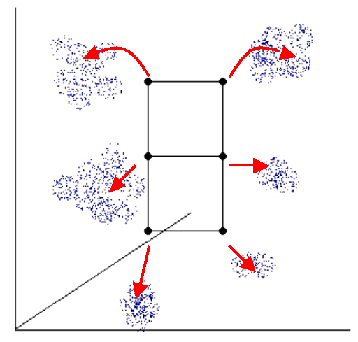
An SOM has a set of nodes with a simple topology (e.g., two-dimensional grid) and a distance function d(N1,N2) on the nodes. Nodes are mapped into K-dimensional "gene expression" space (in which the i-th coordinate represents the expression level in the i-th sample, K is the number of experiments (fields)). The process of mapping is iterative (see Fig.1).

Fig. 1. The diagram shows the principle of iterative clustering of high-dimensional data points by SOM algorithm. The SOM structure is shown by black grid, data points in high-dimensional space are shown in blue. The moving of grid nodes to the regions of higher data density are shown in red.

The iterative algorithm allows moving each node to the K-dimensional space regions with higher density of points (genes). In principle, each node will be located near the cluster of genes in the high-dimensional space. The position of node N at iteration i is denoted f_i(N). The initial mapping f₀ is random. On subsequent iterations, a data point P is selected and the node N_P that maps nearest to P is identified. The mapping of nodes is then adjusted by moving points toward P by the formula (Tomayo et al,1999):
f_i+₁(N) = f_i(N) + t(d(N, NP), i) (P - f_i(N)).

To perform calculation user should define the grid size (number of row and column nodes in two-dimensional grid (see Fig.1), set the maximal number of iterations and set the distance type (to calculate distance between node and data points). There are several measures of expression profile distance between two genes:

(1) Euclidean distance. This is the geometric distance in the multidimensional space. It is computed as:

where x_i, x_j are two expression profiles for genes i,j,k is the index of experiment (field), x_ik is the expression value of gene i in the experiment k.

(2) Squared Euclidean distance. The squared Euclidean distance can be implemented in order to place progressively greater weight on objects that are further apart. The squared Euclidian distance is computed as:

(see explanation above). The Euclidian and squared Euclidian distances are computed from raw data (non-standardized), therefore they may be affected by differences in scale among the expression values in different experiments.

(3) Manhattan distance. This distance is the average absolute difference for the set of experiments calculated by the formula
.
In most cases, this distance measure yields results similar to the simple Euclidean distance, for this measure, the effect of single large differences is dampened (since they are not squared).

(4) Chebychev distance. This distance is computed as d_ij = max_k | x_ik - x_ik |. The measure is useful when one wants to define two objects as "different" if they are different on any one of the experiments.

In SelTag all distance measures (1-3) are normalized to the number of fields involved in calculation. This is useful when take into account expression data with missing values.

Other measures involve correlation coefficient r_ij between two expression profiles of genes i and j.

(5) 1-r_ij; This measure keep close profiles with positive correlation coefficients and is useful when one wants to detect co-regulated genes.

(6) 1-|r_ij|; This measure keep close profiles with higher absolute value of correlation coefficients.

(7) 1+r_ij; This measure keep close profiles with negative value of correlation coefficients (anti-correlated).

Three types of correlation are possible for correlation distance option:
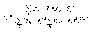
Pearson's r - Pearson's correlation coefficient. The Pearson product moment correlation coefficient between expression profiles i and j is calculated as follows:

where y_ki is the expression level of gene i in the experiment k; is the mean expression level of the gene i. Positive correlation implies that the expression levels of genes i,j are related positively, the higher expression of gene i, the higher expression of gene j. Negative correlation means that the expression levels of genes i,j are related negatively, the higher expression of gene i, the lower expression of gene j. If the r_ij is close to zero, two expression profiles are unrelated.

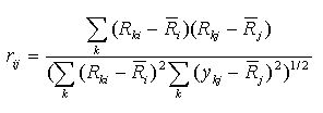
Spearman r - Spearman's correlation coefficient.
This correlation coefficient is computed for ranks. Let R_ki is the rank of the expression level in the experiment k of gene i (relatively to other experiments), R_kj is the rank of the expression level in the experiment k of gene j. Then Spearman's correlation coefficient is calculated by the formula

Kendall's t - Kendall's tau correlation coefficient. To calculate Kendall's t K for data points (y_ki; y_kj) 2K(K - 1) pairs considered (without self-pairing, the points in either order count as one pair). Pairs in which y_ki > y_mi and y_kj > y_mj or y_ki < y_mi and y_kj < y_mj are called concordant pairs (agreement between ranks), pairs with rank disagreement are called discordant pairs. In general, t is calculated as
t = ([number of concordant] - [number of discordant]) / total number of pairs

Example of output data

status=done [0.0 sec]
Number of gene clusters obtained 5.
Cluster Sizes and Scores: 
Cluster 1	1	0.0000
Cluster 2	1	0.0000
Cluster 3	5	0.5954
Cluster 4	14	0.8092
Cluster 5	13	0.8647
List of selected genes, their cluster indices and scores :
No	DataIndex	Name	Cluster	Score
1	1	GEN30482	1	0.0000
2	2	GEN03437	2	0.0000
3	3	GEN03687	3	0.7264
4	4	GEN24649	4	0.9291 

Some lines starting from "status=" are just output the status of the calculation and can be ignored. Then the result cluster information is output: number of clusters, their list with cluster scores. Then list of selected genes with their cluster indices and scores is printed out.