Program package SNNBP (Softberry neural network: back propagation), version 1.0.

The package implements the multi-layer perceptron neural network functions of learning, testing and prediction.

Algorithm description.

The package implements the neural network of the multi-layer perceptron (MLP) topology.
MLP topology description.
The feed-forward neural network model transforms input signals into outputs. The transformation occurs at the neural network units called neurons (Fig. 1). The neuron consists of the weighted summation module (denoted as in the Fig. 1) and non-linear transformation module (denoted as F in the Fig. 1). Such neuron structure is called perceptron.

Fig. 1. The structure of the neuron.

NET is the result of the weighted summation of the input signals xi. OUT is the output of the single neuron, and it is the result of the non-linear transformation by activation function F of the NET value.

where
x={x_i} - the input signals vector,
w={w_i} - weights,
q - bias term,
F - neuron activation function,
NET - weighted sum of the input signals,
OUT - output signal.

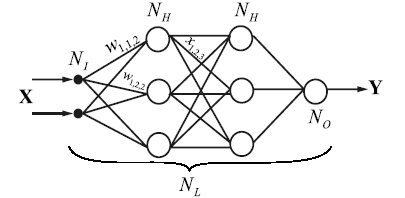
The SNNBP program implements the feed-forward neural network where single units are connected in such way that output of one unit can be input to another unit. In the multi-layer perceptron topology units are combined in sets of layers with no connection of neurons within the layer. Neurons can input signals only from units of the previous layer and forward signals to the units of the next layer (Fig. 2). The number of neurons in the layer is arbitrary and set by user. The number of layers in the network is arbitrary (set by user).

Fig. 2. The structure of the multi-layer perceptron.

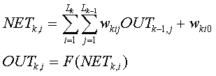
There are three types of layers in such network. Fist is input layer, second is output layer, other layers called hidden. Neurons of the input layer make no transformations, they transmit the input signals to the first hidden layer. The SNNBP implements the algorithm that transformation of the the i-th neuron of the k-th layer as follows:

where NET_k,j is the weighted sum of the inputs for the i-th neuron of the k-th layer (i=1,L_k, L_k - the number of neurons in the k-layer).
OUT_k,j is the output value of the i -th neuron in the k-th layer.
w_ki={w_kij} is the weight matrix, connecting the i-th neuron in the k-layer with the j-th neuron outputs (j=1,L_k-1) of the k-1 -th layer outputs.
w_ki0 is the bias for the i 0^th neuron in the k-th layer.
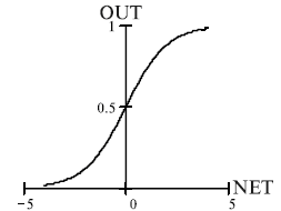
F is the activation function, the current version of the SNNBP program implement sigmoid activation function:

where ñ is the shape parameter (gain) that determines the slope of the sigmoid, when it is close to 0, the slope of the sigmoid is softer, if the gain is large, the shape is close to the step-wise function. The gain parameter is the same for all the neurons in the network.

Fig. 3. The sigmoid activation function.

The SNNBP program allows setting the network topology of the arbitrary size of the input vector, output vector, number of hidden layers and number of neurons per layer. The network topology is set by user, as a rule, the topology can be optimized by trial and error procedure by user. The network with the simple structure may not capture the relationship between the input and output variables sufficiently. The multi-layer perceptron of the large size are more time-consuming to learn and need the large size of the training set to estimate the weights of the network. It is usual practice to start with the simple topology, then add more neurons and control the error after the topology changes.
The network model considers numerical representation of the input and output variables.

It is able to solve the following types of tasks.
1). The non-linear regression or prediction. The neural network is trained to predict the output (target) values using the input value. In most cases, there is one (target) value at the neural network output tan need to be predicted. However multiple outputs can be predicted by SNNBP program also.
2). Classification. The neural network should classify the input sample by its input values into several classes. To code the classes several approaches exist. If it is needed to classify samples into 2 classes, the output of the network can be the single value and the classifying decision is determined by threshold value. Another way is to associate the class value to single output neuron and to select class according to the neuron with maximal output. The last method allows classifying samples into arbitrary number of classes.

The MLP learning procedure.

The idea behind the neural network is that the network can be trained to find the relationships between the input and output data. The learning process assumes the existence of the data for which the true relationship is known (supervised learning). The training data consist of samples for which the relationship between the inputs x and outputs o is known. For the specified network topology, learning procedure selects weights w_ki to minimize error between the outputs of the network and the true output values t (targets).

For the single sample n the targets t are known and the outputs o of the network are calculated (the size of the output and target vectors are equal to M), then the error can be estimated as follows:

For the N samples total error estimate is

The learning task for the neural network is formulated as to fond the network topology and corresponding network parameters (weights) with the minimal value E for some training data set.

This is the optimization problem. For neural network it can be solved numerically by steepest gradient method. The overall optimization scheme is as follows:
1). Set initial weight values if the MLP by random values [-0.5; 0.5].
2). Calculate the gradient direction.
3). Change the weight values wk_ij (and biases w_ki0) for the a -d_kij, where a - is the step length (learning rate), d_kij is the vector of anti-gradient.
4). Repeat steps 2-3 until the error changes during optimization procedure will be small enough.

The SNNBP program implement slightly different optimization based on the error back-propagation algorithm. This is convenient and fast way for gradient calculation. This algorithm allow to calculate weight changes backward, from last layer to the first, the weights for the L_k level are calculated using the error estimates for the neurons in the L_k+1 level. This allows to calculate all the weight changes recursively. The estimate of the gradient is possible in such a way that samples presented to the neural network sequentially. The learning process is divided to the "epochs", during the epoch all the samples from the training data are presented to the neural network. This is so-called batch training option.

The learning algorithm work as follows.
1). Set initial weight values if the MLP by random values [-0.5; 0.5].
2). Present the sample n from the training data to the network.
3). Calculate the outputs o of the NN for the inputs x of the sample.
4). Calculate the error between the outputs o and targets t for the sample n.
5). Using the backpropagation algorithm estimates the gradient are calculated and change the neural network weights according the gradient values are made.
6). Repeat steps 2-5 for all the samples from the training data.
In this procedure, samples are presented to the network randomly during the epoch. The overall learning cycle consisted of the several epochs usually. The number of epochs per learning step is defined by user and selected by trial and error procedure.

Momentum.
Usually, the gradient vector is estimated for current values of the network weights. The step length in the anti-gradient direction is a. In some cases the optimization efficiency can be improved by adding to the descent vector at the current step the vector at the previous step with some coefficient (momentum). This allows searching optimum efficiently in the narrow ravines of the error surfaces. In this case the weight w_kij changes (and w_ki0) made by the value a (d_kij + d_kij(previous)*m), where a - descent step length (learning rate), d_kij is the gradient direction at the current step, d_kij(previous) is the anti-gradient direction at the previous step, m is momentum (ranges from 0 to 1). If the moment is equal to 0, the descent direction vector is determined from the current weight values.

The learning protocol with early stopping.
If the network topology contains many weight parameters, it can over-fit the data in the learning process. This means that the network can recognize the data on which it was trained and cannot make generalizations for another data. This occur when the training data size is insufficient to fit the large number of parameters. To overcome the problem the early stopping procedure is implemented in the course of learning.
The protocol requires additional set of data, validating data set. These data serve as additional check for stop learning process, if the error became increasing on the validating data. The protocol for earsly stopping is as follows.
1). The number of training steps Nsteps is set.
2). At the each step the process of the learning by user-defined number of epochs is performed as described previously.
3). After each step the error of the NN is estimated on the validating data. If the error is less than was obtained previously, the network parameters are saved.
4). Otherwise the learning process continues until the number of learning steps is less than Nsteps or the error on the validating data is too large (say, 2 times larger than the minimal error obtained in previous steps). This process always saves the network parameters, which give the minimal error obtained during learning process for the validating data. The threshold parameter for large error deviation is set by the user.
The error on the training data in this protocol usually decreases to the small value and became fluctuating after some steps of learning. The error on the validating data is also decreasing after some steps, but at some point it may became increasing (the point where over-fitting occur). This protocol allows overcoming the over-fitting problem efficiently.

The SNNBP options.

The SNNBP program allows three options: learning, testing and prediction.

First option (SNNBP -Learn) implement the back-propagation training algorithm and output the optimal NN structure, saved in the SNNBP internal format. It is also possible to save the network parameters in the C file that can be compiled as a separate module that implements the NN evaluation by C-function. It also implement some additional features:

• Internal normalization. After reading all the data are normalized in such a way that variables are scaled to the interval [0.1;0.9]. There is no need in data normalization by user. The neural network prediction values are rescaled back after prediction to the initial data range.
• Prediction output. The program may save predicted values obtained by best network parameters for the training, validating and the testing data.

Second, testing option (SNNBP-Test) implement testing of the previously obtained network on the user data. The file should contain both input and output values. The error estimate is printed out. User can also output predicted values (outputs) for test data into user-defined file.

Third, prediction option (SNNBP-Predict) is implemented. In this option neural network calculate output values (predictions) using input values from the data file (target values need not be specified in this option). The predicted values are saved into user-defined file. The error is not calculated in this option.